
Introduction
Exhaust headers serve to optimize the pulsatile flow of exhaust gases from the internal combustion engine by means of resonance tuning to increase the air mass flow rate and thus the power of the engine. The resonance characteristics of the quarter wave primary tubes is of highest importance.
In a naturally aspirated engine, one without forced induction from a turbocharger or supercharger, the engine working as a positive displacement air pump moving the air into and out of the engine. The intake stroke of the engine creates low pressure inside the cylinders, which causes air to flow due to the pressure difference inside the cylinders and atmospheric pressure. After the compression and combustion strokes, the exhaust valve is opened while the cylinder pushes exhaust gasses out in discrete periodic pulses. These nature and intensity of these exhaust pulses can be analogized to shotgun blast waves where each pulse is expelled at high velocity and momentum. While most of the exhaust gasses are expelled during the exhaust stroke some of the spent exhaust gasses can remain in the cylinder due to the flow resistance, or pressure drop, of the exhaust system and atmospheric pressure.
In some engines, for emissions reasons, exhaust gasses are intentionally left in the cylinder for charge air dilution to reduce combustion temperatures and smog forming NOx. This can be achieved through restrictive exhaust designs and proper adjustments of the intake and exhaust valve timing. While effective at reducing emissions, this comes at the cost of reduced engine power.
If the design goal is to increase engine power for race applications, the spent exhaust gasses should be scavenged from the cylinders to the greatest extent possible. This will allow more fresh air to be drawn in during the next intake stroke. Higher mass flow rates of exhaust leaving the engine means more air can flow into the cylinders to allow more fuel to be burned and more power to be produced. To understand how to increase scavenging, we must first consider the transient nature of the exhaust pulse waves and how to synchronize the acoustic resonance as a means of scavenging exhaust from the engine.
Exhaust Pulses and Scavenging
The stream of gases exiting the engine is not continuous, instead it is separated into discrete pulses as the exhaust valve opens and closes. The pressure at the inlet of the exhaust headers starts at atmospheric pressure, then the valve opens, and pressure quickly increases as the exhaust rushes out into the stagnant air inside the primary header tubes. The stagnant air resists the sudden change in velocity due to the difference in momentum but once the blast of high velocity gasses is set into motion it tends to stay in motion, even when the exhaust valve closes. After the exhaust valve closes the pressure at the header inlet drops since the flow resists slowing down from its high velocity, again due to momentum of the gases in motion. It is this momentary low pressure which can be utilized to scavenge exhaust gasses from other cylinders for increased power.
In an engine with multiple cylinders, the low-pressure waves from the end of the exhaust pulse of one cylinder can be routed to the next cylinder and help vent its gases more easily. This effect is commonly called scavenging. In order to design a system to use scavenging, the paths of the outlet gases must combine together so that one cylinder can experience the low pressure of another. This is done in a manifold or a merge collector where the gases combine and continue in a single tube towards the muffler. However, this low-pressure event only lasts so long before returning to atmospheric pressure, so the timing of when the low-pressure wave reaches the next cylinder must be carefully controlled. This is where Long Tube Headers come in. Each of the primary tubes is a quarter wave acoustic resonator. The resonant frequency is determined by the primary tube’s length and diameter in addition to the properties of the exhaust gas including temperature, molecular weight, and ratio of specific heats (gamma).
Well-designed Long Tube Headers will generally start with small diameter primaries close to the engine with gradually increasing diameters as distance from the engine increases. The goal is to maximize exhaust velocity without creating excessive pressure drop. Overall, the design is a balancing act of length, diameter, pressure drop and frequency(s). The optimum configuration can be found on the dyno with extensive fabrication and testing but much of the initial design phase can be performed in computer simulations.
Solidworks Flow Simulation
Solidworks is a solid modeling computer-aided design (CAD) program with the addon Solidworks Flow Simulation, which is a computational fluid dynamics (CFD) program with the ability to simulate liquid and gas flows inside or outside a model and calculate performance metrics to be used for design. In order to model the time dependent nature of exhaust pulses in exhaust tubes, a transient simulation must be used. Furthermore, nested iterations must be used to properly capture transient compressibility effects such as transient shock waves and acoustic waves [2]. Without nested iterations, the solve will not show much compressibility, and the lowest pressures will appear to be near perfect vacuums. The fluid used in this simulation is exhaust gas at 1200K. The gas is able to experience both laminar and turbulent flow conditions.
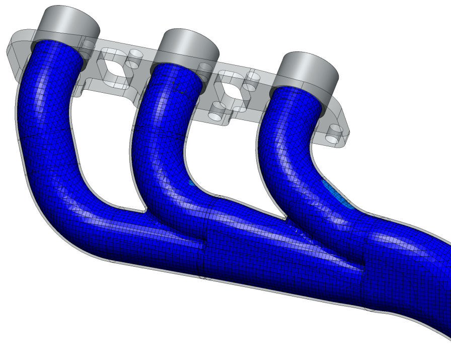
Setup
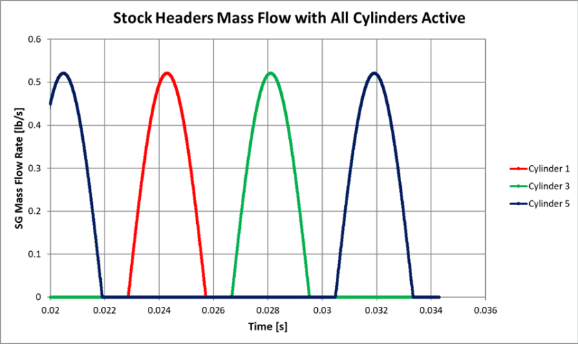
The stock exhaust headers were modeled into Solidworks and a second variation was created with Motordyne Engineering 370Z Long Tube Headers with Straight Pipe (see Figure 1 and 2). Both models’ driver side exhaust header was mirrored onto the passenger’s side for simplicity. The boundary conditions are six mass flow inlets and two static pressure outlets. Each of these boundary conditions has data taken and recorded as a surface goal (SG). These boundary conditions are labeled in Figure 3. The inlet mass flows are important to focus on because Solidworks Flow Simulation and other CFD packages cannot simulate motion of a valve opening and closing since the mesh utilized in a finite element analysis is static. However, Solidworks can make this mass flow inlet vary in magnitude with time. Thus, a simple sinusoidal curve was generated to represent the opening and closing of this valve. It is noteworthy to identify that this simple of a mass flow is not entirely correct. The curve is exactly one fourth of a full revolution of the internal combustion engine which depending on the level of valve overlap and other tuning might be smaller or larger. Also with a sinusoidal mass flow, the mass flow is mirrored across the peak flow rate, which is not entirely true since the pressure inside the cylinder would be higher on the left hand side of this peak than the right hand side, and therefore the left side would have more mass flow than the right. However, it does correctly show the concave down nature of the mass flow: as the piston moves from bottom dead center (BDC) to top dead center (TDC) the mass flow slowly increases, peaks, then decreases.


The equation below in Figure 4 show the simplified mass flow used for the CFD simulations. A is the amplitude of the sine wave in pounds per second, f is the frequency of the sine wave in Hz, t is time in seconds, φ is the phase shift in radians and n is the cylinder number, starting at 0 for the first cylinder and incrementing up for each following cylinder. The frequency (Figure 5) can be found from the design point engine RPM and the engine setup. The phase shift (Figure 6) is a function of the number of cylinders (n) and whether it is a four stroke or two stroke cycle. This phase shift is then applied to each cylinder’s mass flow function in the firing order of the engine. The amplitude calculated by taking real world dyno results to get the mass flow of exhaust gases in one cylinder (Figure 8) and dividing it by the number of cylinders and solving for A in the integral in Figure 6. Measured dyno results of output power (HP), torque (T), RPM and air fuel ratio (AFR) are used in the equation in Figure 9, taken from Garrett’s Turbo Expert [4], to obtain brake specific fuel consumption (BSFC) which is then used to get the mass flow in Figure 8.


Dyno Testing
Previous third-party testing was conducted by Ben Blackwell comparing Motordyne Long Tube Headers to stock headers and stock catalytic converters on a Nissan 370Z. In both of these runs the vehicle already had installed a Motordyne Shockwave Exhaust system. The engine was not retuned after the Motordyne Long Tube Headers were installed. The results are plotted in Figure 10, and a brief portion of the data is tabulated in Table 1. These tests show that the Motordyne Long Tube Headers were able to produce a maximum of 37.23 hp and 27.16 ft*lbs. at 7200 RPM. The air/fuel plot shows that the Motordyne Long Tube Headers achieved these gains at a higher AFR. These gains were most likely due to an increased airflow caused by the removal of the backpressure caused by the stock catalytic converter and the further decreased pressure due to scavenging on the Motordyne Long Tube Headers.
Table 1: Brief Results from Ben Blackwell of Stock Headers vs Motordyne Long Tube Headers
Stock Headers | Motordyne Long Tube Headers | Percent Increase | ||||||
RPM | HP | TQ | AFR | HP | TQ | AFR | HP | TQ |
3100 | 127.9 | 216.7 | 12.6 | 140.1 | 237.3 | 13.2 | 9.5% | 9.5% |
3500 | 153.5 | 230.4 | 12.4 | 160.3 | 240.5 | 13.1 | 4.4% | 4.4% |
4000 | 174.7 | 229.4 | 12.0 | 184.6 | 242.4 | 12.8 | 5.7% | 5.7% |
4500 | 198.6 | 231.8 | 11.9 | 204.5 | 238.6 | 12.7 | 3.0% | 3.0% |
5000 | 217.4 | 227.0 | 11.8 | 235.0 | 246.9 | 12.8 | 8.1% | 8.7% |
5500 | 236.6 | 225.9 | 11.6 | 252.9 | 241.5 | 12.7 | 6.9% | 6.9% |
6000 | 252.0 | 220.6 | 11.5 | 275.1 | 240.8 | 12.6 | 9.2% | 9.2% |
6500 | 267.2 | 215.9 | 11.5 | 293.9 | 237.4 | 12.7 | 10.0% | 10.0% |
7000 | 278.0 | 208.6 | 11.5 | 310.6 | 233.0 | 12.7 | 11.7% | 11.7% |
Another similar third-party set of testing was conducted by Dynosty comparing the stock headers against Motordyne Long Tube headers. Both systems used Motordyne ART pipes and Motordyne Shockwave cat back exhausts. The dynamometer results showed a 13.2 Hp gain in max power on the Motordyne Long Tube headers without tuning and a 25.14 Hp gain with tuning. See reference [1] for details.

Steady State Simulations
The first simulation was a comparison of stock headers with Motordyne Test Pipes and a Shockwave Exhaust (see above Figure 1) and Motordyne Long Tube Headers (see above Figure 2). This simulation was conducted in a steady state scenario unlike the rest of the simulations. The mesh of these two simulations is shown in Figures 11 and 12. This was done to show the pressure increase above atmospheric pressure (14.696 psi) at a constant mass flow of 0.08291 lb/s in each cylinder. The mass flow was calculated using the equations in Figure 7 and 8 and Ben Blackwell’s results. The steady state approach allows us to isolate the pressure drop of the geometry from the resonant pressure waves occurring in a transient simulation. The resultant data is tabulated below in Table 2. Notice that the stock headers have the highest pressure in the farthest forward cylinder, but the Motordyne Long Tube Headers have similar pressures in all cylinders. Ideally for tuning purposes each cylinder would experience the same pressure.
Table 2: Steady State CFD Static Pressure
Cylinder | Static Pressure (psi) | |||
Number | Stock Headers | Percent above Atmospheric Pressure | Motordyne Long Tube Headers | Percent above Atmospheric Pressure |
1 | 16.67 | 12.6% | 15.66 | 6.4% |
2 | 16.68 | 12.6% | 15.67 | 6.4% |
3 | 17.04 | 14.8% | 15.61 | 6.0% |
4 | 17.04 | 14.8% | 15.61 | 6.0% |
5 | 17.36 | 16.6% | 15.60 | 6.0% |
6 | 17.36 | 16.6% | 15.60 | 6.0% |


Transient Simulations
The second simulation was a transient simulation conducted on the Motordyne Long Tube headers, however, only one cylinder is active, as if the engine only routed only one exhaust port to the headers. This was done to see one individual exhaust pulse and its effect on the pressures of the other cylinders. The mesh and other parameters listed in Table 3 are used for all the transient simulations. The simulation was repeated for three full pulses of cylinder 5, which as seen from Figure 3 above is the furthest forward cylinder on the left-hand side of the engine. Three full cycles represent six revolutions of the four-stroke internal combustion engine. The plotted data only shows the latter half of these three pulses, since the simulation needs to build up initial flow patterns that will be repeated in subsequent time periods. The sinusoidal mass flow through each header is shown in Figure 13, the velocity in Figure 14, the dynamic pressure in Figure 15 and the static pressure in Figure 16. The mass flow shows distinct sinusoidal starts and stops. The time that this pulse took to reach the other cylinders is seen as a delay in the static pressure graph. After the initial peak static pressure of approximately 27 psia on cylinder 5, the pulse quickly drops in static pressure to nearly 10 psia at 0.023 seconds. At 0.025 seconds, cylinders 1 and 3 both experience this static pressure that is lower than atmospheric. This is the time when the next pulse should occur to maximize scavenging. Notice there is another peak in pressure in cylinder 5 at 0.026 seconds and then another dip in pressure at 0.028 seconds which is the pressure wave reflecting back on itself as it attempts to return to atmospheric pressure in a damped sine wave fashion.
Table 3: Information of the Transient Simulations
Stock Headers | Long Tube Headers | |
Mesh Cell Count | 144,050 | 142,961 |
Iterations | 4,200 | 4,200 |
Time Step | 8.1633e-06 s | 8.1633e-06 s |
Engine RPM | 7,000 RPM | 7,000 RPM |
Peak Mass flow | 0.52 lb/s | 0.52 lb/s |


The next simulation is with all six inlets active while using the same Motordyne Long Tube headers. Same as before the simulation was run through three full cycles, or six revolutions. The sinusoidal mass flow through each header is shown in Figure 17, the velocity in Figure 18, the dynamic pressure in Figure 19 and the static pressure in Figure 20. A second static pressure plot is shown in Figure 21 that includes both left and right-hand sides, however with all six lines it becomes hard to differentiate. Looking at Figure 20, the maximum pressure the peaks experience is slightly higher by 2 psi than in the previous simulation with only one cylinder active (Figure 16), which agrees with the higher total mass flow throughout the system and lowest troughs in static pressure are also lower by about 2 psi. The dynamic pressure and velocity peaks are slightly lower than the single active cylinder simulation, indicating a greater amount of energy was put into static pressure rather than movement. The sharp transition bump in static pressure that happens right before cylinder 5 opens near 0.03 seconds is slightly smaller now that all cylinders are active, since the trough lowest point before this pulse was at 0.028 seconds with only one cylinder active but now is at 0.029 seconds, due to cylinder 1 firing. This timing is due to the velocity difference: the faster gases in the simulation with only one cylinder active reached the next cylinder quicker than this current simulation. The smaller this bump is the better, since it indicates how closely aligned the lengths of the long tube headers are to optimal, ideally the valve would open closer to the lowest trough of the static pressure, maximizing the utility of this low pressure time period.


The third transient simulation switches to the stock headers with Motordyne Test Pipes and a Motordyne Shockwave exhaust, so as to only change the headers themselves. The stock catalytic converters were removed due to the difficulty of modeling this porous area accurately. The graph of mass flow is shown in Figure 22, the velocity in Figure 23, the dynamic pressure in Figure 24 and the static pressure is shown in Figure 25. The maximum peak pressures were lower than the long tube headers by about 4 psi, instead the dynamic pressure and velocity peaks are much higher on these stock headers. The smaller tubing in these stock headers forces the exhaust gases to move faster thus having much greater dynamic pressure instead of static pressure. The time delay that it took one cylinder to experience the pressure of another cylinder was lower down to approximately 0.001 seconds, since the path length the air would have to travel is much shorter than on the long tube headers. Thus, the stock headers had their peak static pressure in the active cylinder also was the nearly the same time as the peak pressure in the closed cylinders. The shape of the pressure curves varied greatly from cylinder to cylinder, since, as shown in the first stead state simulation, the geometry of these stock headers creates a less uniform pressure. Cylinder 1 has the smallest static pressure drop as shown from the steady state simulations, therefore it has the highest velocity. However, this pattern does not show up in the static pressure in Figure 25: cylinder 1 had the highest pressure followed by cylinder 5 then cylinder 3. If we instead look two revolutions back in Figure 26 at time 0.12 seconds the peak of cylinder one is the lowest, where we might expect it to be, so the peak at 0.025 seconds might be an outlier caused by an interaction of previous pressure waves.


The most important pattern to note is the sharp trough in the stock header’s pressure plot (Figure 25) before the valve opens on the active cylinder: the pressure here is only below atmospheric for a very short interval, less than 0.001 seconds whereas the long tube headers (Figure 20) experience a static pressure below atmospheric for almost twice as much, approximately 0.002 seconds. If we were to characterize the amount of area below atmospheric pressure and the pressure curve as a gauge of the length of time the pressure stayed below atmospheric along with the magnitude of this pressure, the stock headers have a much lower value of 0.0039 versus the long tube headers value of 0.0067. This value shows us that the stock headers remained below atmospheric for less time, which is worse for performance since the ideal case is the lowest pressure possible for the longest time in order to push out more air from the exhaust manifold. The shape of the curve is also much sharper with many large jumps from high to low pressure, which could indicate more turbulent losses as the flow changes direction more often.
Conclusion
Stock headers of a Nissan 370z have been compared to Motordyne Long Tube Headers on dynamometer and in a CFD simulation with Solidworks Flow Simulation. The dynamometer results show that the Motordyne Long Tube headers increased horsepower and torque output of the engine by as much as 11.7%. The steady state simulations show Motordyne Long Tube Headers have a lower pressure drop across the length of the exhaust system by as much as 1.76 psi as well as more equal pressure in each cylinder as apposed to the stock headers. The transient simulation shows the shape of a pressure pulse over time as experienced by the exhaust header. Higher peak static pressures were observed in the long tube headers than the stock headers as well as lower minimums. However, the stock headers experienced larger fluctuations in pressure due to the shorter length. The stock headers also experienced much higher velocities and dynamic pressures at all points than the Motordyne Long Tube Headers, indicating better pressure recovery from the Motordyne Long Tube Headers. The simulations shown here are the first step in the design process of tuning long tube header designs.
References
[1] Motordyne Headers on Nissan 370Z Dynosty Tuned 328WHP. Dynosty, 2016. https://youtu.be/zcLMeQUyh0U.
[2] “Solidworks Flow Simulation 2020 Technical Reference.” Dassault Systemes, November 14, 2019.
[3] Teja MA, Ayyappa K, Katam S, Anusha P (2016) Analysis of Exhaust Manifold using Computational Fluid Dynamics. Fluid Mech Open Acc 3: 129.
[4] “Turbo Tech 103 Expert: Compressor Mapping.” Garrett Motion, January 7, 2020.